The 3W’s of RNN — What, Why, and Working


Photo by Jeffrey Brandjes
RNNs are feedforward neural networks deep down but with a catch, i.e., they have memory
Definition:
RNNs are a class of Neural Networks that work on modelling sequential data. Recurrent Neural Networks use their reasoning from previous experiences to inform the upcoming events with the help of internal memory.
Why RNNs?
Before answering that, let me give an intuition on the importance of memory during predicting a sequence
Let’s take a sentence:
Usain Bolt, an eight-time Olympic gold medallist, is from ___
If I ask you to fill in the blank, your answer might probably be ‘Jamaica’ or ‘North America’. But what made you come up with those answers?
It’s the word ‘Usain Bolt’. This example illustrates the importance of memory in predicting a word.
Imagine using an ANN to fill the blank. It would predict the next word with just the help of ‘from’, which can be gibberish. But RNNs remember what they saw earlier, making them capable of producing a reasonably accurate answer.
Well, how does a Neural Network have memory?
An RNN calculates hidden state value based on the current input and previous timestep’s hidden state. In simple words, whatever happened in the previous timestep affects the current output. This is basically remembering something and using it when needed.
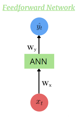
Feedforward Network (ANN)
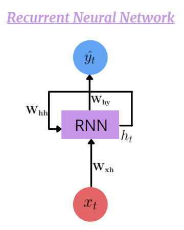
Recurrent Neural Network (RNN)
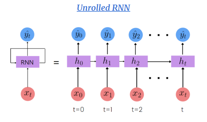
RNN unrolled in time
A RNN representation is NOT multiple layers of ANN, rather a single ANN at multiple timesteps
Working
Forward Pass-
At time t,


As we can observe here, the hidden state is dependent on the current input and the previous timestep’s hidden state
At each time step t, only the Hidden State (h) keeps updating while the Function (F) and Weights (W) stay the same
Common activation functions ‘F’ are — Tanh, RelU, Sigmoid
Loss-
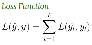
The loss function for an RNN is defined as the sum of individual loss values of each timestep
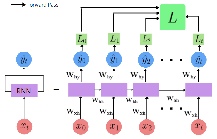
Forward Pass and Loss
Backpropagation Through Time (BPTT)-
Backpropagation is done at each point in time. At timestep T, the derivative of the loss L with respect to weight matrix W is expressed as follows
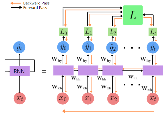
Backpropagation Through Time
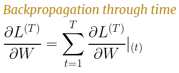
In a simple feedforward system, the gradient of the loss is calculated for each parameter.
The same happens here, but it happens for each timestep as all timesteps together contribute to the total loss.
And as each time step is dependent on the previous timestep, calculating the gradient for timestep, say t, would require gradients of t=0 till t=t-1.
If you’re able to follow till here, YOU’RE DOING AMAZING.
But we have 2 new villains here. They are Exploding and Vanishing gradients. During BPTT, we have to multiply multiple gradients. For example, calculating for t=15 would require multiplying 15 gradient values
Exploding Gradients:
Happens when many gradient values > 1
Multiplying large numbers results in an even bigger output which leads to drastic value updates
Eg. 10 5 10 * 7= 3500
VanishingGradients:
Happens when many gradient values < 1
Multiplying small numbers results in an even smaller output which has no significant effect while updating values
Eg. 0.01 0.5 0.1 * 0.01 = 0.000005
So it is evident that RNNs are useful in figuring out small sequences. But it fails when it encounters a large sequence. That is, it has short term memory.
Here is where gated cells come in.
LSTMs and GRUs were implemented to tackle the short term memory problem. These networks are very complex and have a long term memory making them very efficient in long sequences.
Implementing RNN:
I will be implementing RNN using Pytorch as it is easier to understand everything that’s happening under the hood.
- Define a class and the constructor
2. Create a function to generate a hidden layer for the first pass
3. Create a ‘forward’ function that defines the flow of data.
Create an initial hidden state
Pass input and hidden state to RNN
Flatten the output
Pass output to dense layer and get the prediction
All Together -
Training (Illustration without actual data)**-**
This model takes 28 dimension input (28 unique words in the dictionary), has 12 dimensions in hidden layer and produces 10 dimension output. After applying softmax, taking the class with the highest probability gives us the predicted word
I hope this article was able to provide what you were looking for and help you in your Deep Learning journey. Do drop down your reviews and share this along :)
Further Reading
Illustrated guide to RNNs - Video
The Unreasonable Effectiveness of Recurrent Neural Networks - Blog
Bonus :)
See ya with another article. Thank you for giving this a read ❤

