Why BFGS over Gradient Descent

Function optimization done right
Photo by Armand Khoury on Unsplash
BFGS falls into the category of optimization algorithms based on Quasi-Newton approaches.
Where and how it is used
BFGS is a type of second order optimization algorithm. BFGS has usages in machine learning in algorithms such as logistic regression etc. It’s main usage is in the necessary minimization of cost function in a machine learning algorithm, in order to correctly find the best approximation algorithm required of the model.
So what is a Quasi-Newton approach?
Basically, according to Newton’s method for finding roots of a function with multiple variables, any function can be categorized as given below,

where the Jacobian matrix is given as,

Any Newtonian method where the Jacobian matrix is replaced with an approximation is considered a Quasi Newtonian method.
Why Newtonian methods are preferred over Gradient Descent
As you might know, in Gradient descent, we intend to minimize a given cost function, depicted as,

Here α is the learning rate of the Gradient descent function.
Here the action of the Gradient Descent function depends solely on the parameter of the derivative of the function, hence categorizing this method as a first order optimization method. Although this method is a good way to optimize a given cost function, as we work with local and limited information at each step linearly, this leads to certain limitations to it.
Therefore, we look towards a more efficient method requiring and analyzing more information and parameters, i.e. a second order optimization method.
Newton’s method
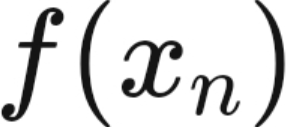
Consider a function f(x), with a corresponding step size of ε.
According to Taylor approximation, approximation of the function at the given step would be,

The required function would be minimized when the below value equates to 0.

Hence the value of ε will come out as,

As we can see, unlike in first order optimization, here the value of step size analyses and considers second order behavior of the required function.
Iteration will be as follows,

Now, in the case of multiple dimensions,
The first derivative is replaced by the gradient of the function
and the second derivative is replaced by the Hessian H.
i.e.


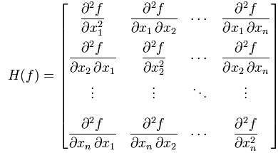
Hessian H of a function is defined as a matrix of partial second order derivatives of f.
i.e.

So finally, for multiple dimensions n, the iterative scheme would be

This method generally yields a very high optimization rate, far higher than that of gradient descent.
So why not always use Newton’s method?
There are certain disadvantages to it:
a. Newton methods can only be used if function is twice differentiable.
b. The method works only for convergent functions and isn’t effective in optimization in the case of multiple curvature optimization requirements, for eg: neural networks.
c. The main disadvantage is that, for each iteration of Newton’s method, it requires solving a large linear system of equations, which for large scale problems can be highly computationally expensive. Computing and analyzing the Hessian H tends to require prohibitively high amounts of time.
In comes Quasi Newton methods!
The essence of a Quasi Newton method is to be able to provide computational sustainability by reducing calculation and iteration costs at each optimization step. This is achieved by simply approximating the Hessian H in the iteration step instead of actually computing the whole exact value.
The value of the approximation is denoted as B, and at each iteration n+1, the new Hessian approximation B is obtained using previous gradient information.
BFGS
Now, for using a Quasi Newton method for optimization, certain constraints need to be put for the Hessian approximation, B, to be calculated.
One of these constraint methods is called the BFGS method, named after it’s creators: Broyden, Fletcher, Goldfarb, and Shanno.
The constraints are as follows:
a. B at every successive step should be considerably close to it’s previous step value, hence, we intend to minimize the difference between them, i.e.

b. “ Matrix Norm” is the mathematical term to categorize the closeness between two values, in BFGS, Frobenius norm is chosen to work upon. Using this method, the iterative value of B comes out in the form of,

where, U and V are symmetric first rank matrices.
c. U, V and inversion of B is found out using a method called, Woodbury’s formula and therefore, results in further iterations being completely relieved of recalculation and inversion of the Hessian H, hence resulting in a faster and more efficient method for function optimization.

Implementation
Lets start by defining a function first (constants defined by array)
Then let’s write a function for it’s derivative
Finally, let’s use the BFGS method to optimize it, giving in the necessary values
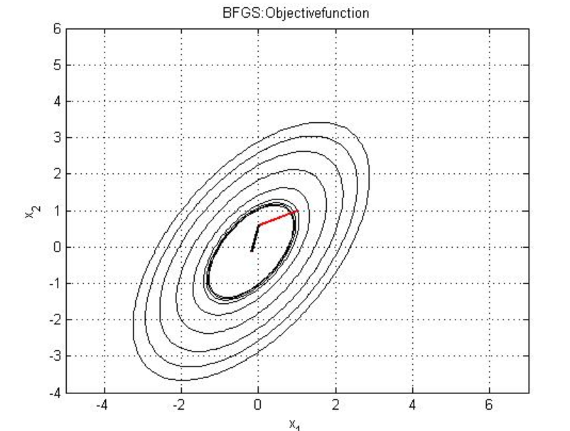
The output will look like this,

Thank you for reading this article, I hope that I was able to provide some insight into understanding and using this algorithm.
Do feel free to contact me at my social handles;


